

Inverse Liquid Chromatography (ILC)
Principle
Since the beginning, chromatography was also applied in order to carry out physicochemical characterizations. The earliest mention of physicochemical measurements by gas chromatography was in 1947, when Glueckauf pointed out that adsorption isotherms could be determined from the breakthrough curves of gas-solid chromatography.
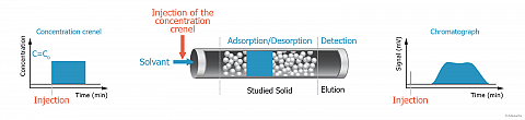
For such purpose, the adsorbent (solid to investigate) is used as packing material for the column instead of the classical chromatographic phase. The adsorption capacity of the adsorbent is then evaluated by injecting a chosen adsorbate. In other words, the adsorbate plays the role of a molecular probe.
Because of the inversion of the respective role of the mobile and the stationary phase, this kind of chromatography is called “Inverse Chromatography”.
We may distinguish several “Inverse Chromatography” techniques depending on the used mobile phase (gas or liquid) and on the amounts of injected molecular probes.
When a liquid is used as carrier phase, the corresponding Inverse Chromatography technique is called Inverse Liquid Chromatography (ILC).
This technique offers a dynamic way to study the adsorption in liquid media of various molecular probes onto powders, particles or fibers. Low molecular weight molecules, but also macromolecules or surfactants could be used as probes.
The obtained informations are:
- adsorption isotherms,
- desorption isotherms,
- the amount of irreversible adsorbed probes.
Irreversible adsorption
In some cases, strong solute adsorption can arise. This could result either from chemical reactions occurring between the solute and the adsorbent surface or by strong physisorption of the solute on the adsorbent.
Such a phenomenon is observed on the figure, here above, that compares the chromatograms obtained after two successive identical injections of the same solute (presently octyltriethoxysilane) on silica. We notice that the desorption profile of both chromatograms is identical. In contrast, their adsorption profile looks very different.
Generally, the second and the next injections give reproducible chromatograms. But when “irreversible“ adsorption occurs, the first injection gives a narrower chromatogram. Since, the chromatogram areas are proportional to the eluted solute amount, we can conclude that the chromatogram area difference corresponds to the “irreversibly“ adsorbed solute amount. On the figure, this amount is depicted in grey.

Reversible desorption isotherm
The most common way to determine desorption isotherms is to practice the so called “frontal chromatography”.
In such experiments, the desorption profile, or rear boundary, is obtained at the adsorption equilibrium and may therefore be used to compute the isotherm. Hence, at each point of the rear boundary, an equilibrium concentration $C$ and the corresponding adsorbed amounts $Q_{ads}$ are determined. The amount adsorbed is calculated by computation of the area under the peak, starting from the tail end ($C=0$).$$Q_{ads} = \int_{0}^{C} (V-V_0).dC$$
where $Q_{ads}$ is the amount of compound adsorbed by 1g of the column packing, under equilibrium at concentration $C$ and $V$ and $V_0$ are the retention volumes, corresponding to the point of the diffuse profile, at concentration $C$, or characteristic point, respectively of the experimental profile and for the theoretical injection profile.
Thus, each point of the rear profile gives one point of the isotherm.
In a same manner, isotherms of adsorption can also be measured. However, for that purpose, the injection profile must be changed. The use of a gradient of concentration is probably the best adapted profile.
In order to get further information, the obtained curves were fitted assuming an isotherm model. The most used remain the single Langmuir type isotherm model. The following relation describes this model:$$Q_{ads}=Q_0.\frac {b.C}{1+b.C}$$
This model supposes a homogeneous surface from a point of view of its properties and also a maximum adsorbed quantity limited to a monolayer of adsorbed molecules ($Q_0$).
The mathematical tools make it possible to find easily the values of the parameters $b$ and $Q_0$ that best describe the experimental isotherms.
However, it happens that the Langmuir model describes only imperfectly the isotherms. In such cases, one calls upon other models.
These models are:
- The bi-Langmuir model: $Q_{ads}=Q_{0,1}.\frac {b_1.C}{1+b_1.C}+Q_{0,2}.\frac {b_2.C}{1+b_2.C}$ with $Q_0=Q_{0,1}+Q_{0,2}$
- The Freundlich model: $Q_{ads}=k.C^{\frac {1}{n}}$ where $k$ is a constant and $n$ a heterogeneity factor.
- The Redlich-Peterson model: $Q_{ads}=\frac {k_R}{1+a_R.C_\beta}$ where $k_R$, $a_R$ and $\beta$ are constants ($0≤\beta ≤1$).
Advantages and limitations of ILC
Advantages:
- Determination of adsorption and desorption isotherms in a unique experimental run.
- Irreversible adsorbed probe amounts determination ( ).
- Only few sample, probes and solvent amounts are needed for such determinations (compared to static methods).
- Quick determination of the isotherms once the protocol drawn up.
- Experiment conditions often close to the industrial process.
Limitations:
- Protocols sometimes long and delicate to develop.
- Sensitivity of the detectors.
- Solvent’s cut-off sometimes handicapping (UV).
- Variations between probe’s and solvent’s refractive indexes sometimes too weak.